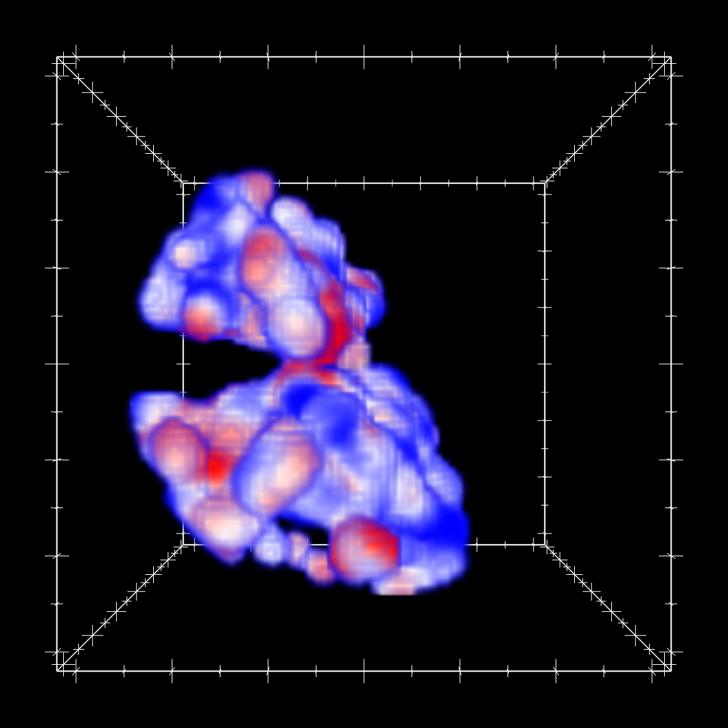
 Above: 2D snapshots of the smoothed 6dFGSv peculiar velocity field in 3D, plotted on a grid in supergalactic cartesian coordinates, with gridpoints color-coded by the value of the "logarithmic distance ratio", which is a logarithmic representation of peculiar velocities, with redder colors corresponding to more positive peculiar velocities (motion away from us, once Hubble expansion is removed) and bluer colors corresponding to more negative peculiar velocities (motion towards us, once Hubble expansion is removed). The Milky Way lies at the center of the plot (0, 0, 0), and the box is 320 Mpc/h (1.5 billion light-years) across.
The full 3D version of this plot can be downloaded here. Adobe Reader version 8.0 or higher enables interactive 3D views of the plot, allowing rotation and zoom.
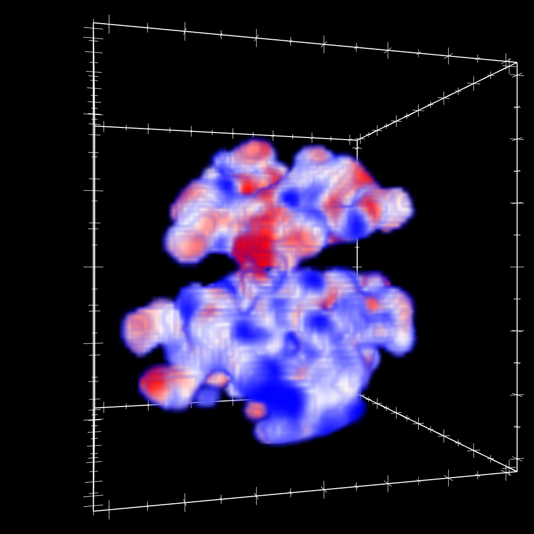
Figure 12: Smoothed 3D velocity field, with supercluster positions superimposed
Above: 2D snapshots of the smoothed 6dFGSv peculiar velocity field in 3D, plotted on a grid in supergalactic cartesian coordinates, with gridpoints color-coded by the value of the "logarithmic distance ratio", which is a logarithmic representation of peculiar velocities, with redder colors corresponding to more positive peculiar velocities (motion away from us, once Hubble expansion is removed) and bluer colors corresponding to more negative peculiar velocities (motion towards us, once Hubble expansion is removed). The Milky Way lies at the center of the plot (0, 0, 0), and the box is 320 Mpc/h (1.5 billion light-years) across.
The full 3D version of this plot can be downloaded here. Adobe Reader version 8.0 or higher enables interactive 3D views of the plot, allowing rotation and zoom.
Figure 12: Smoothed 3D velocity field, with supercluster positions superimposed
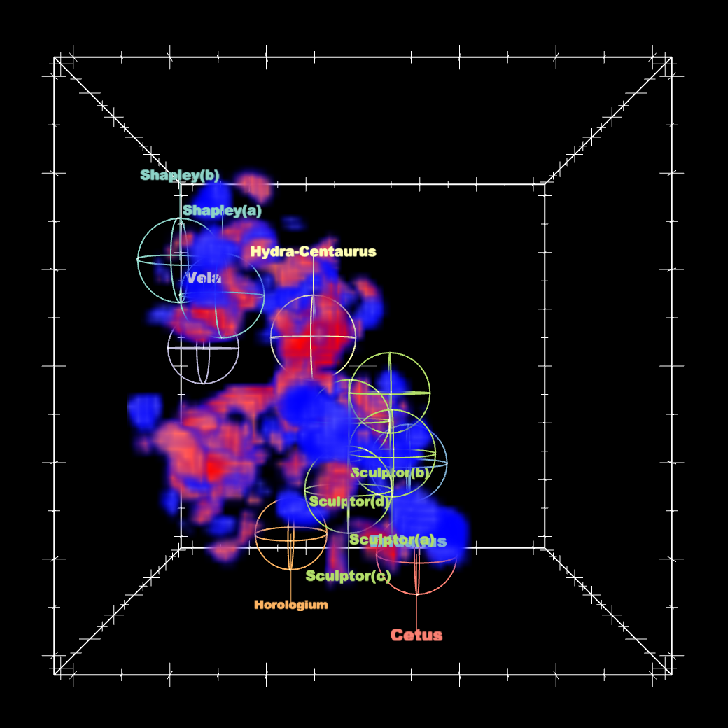
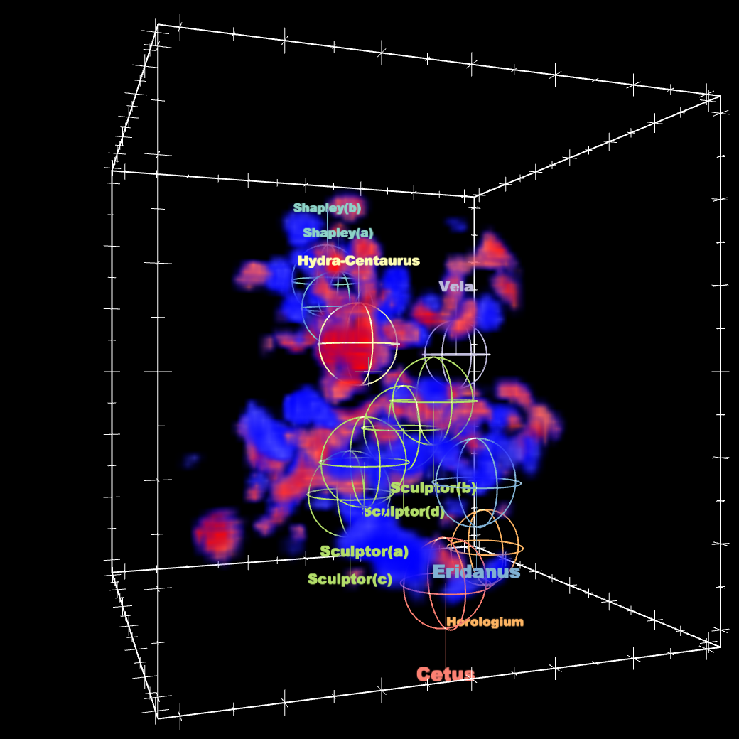
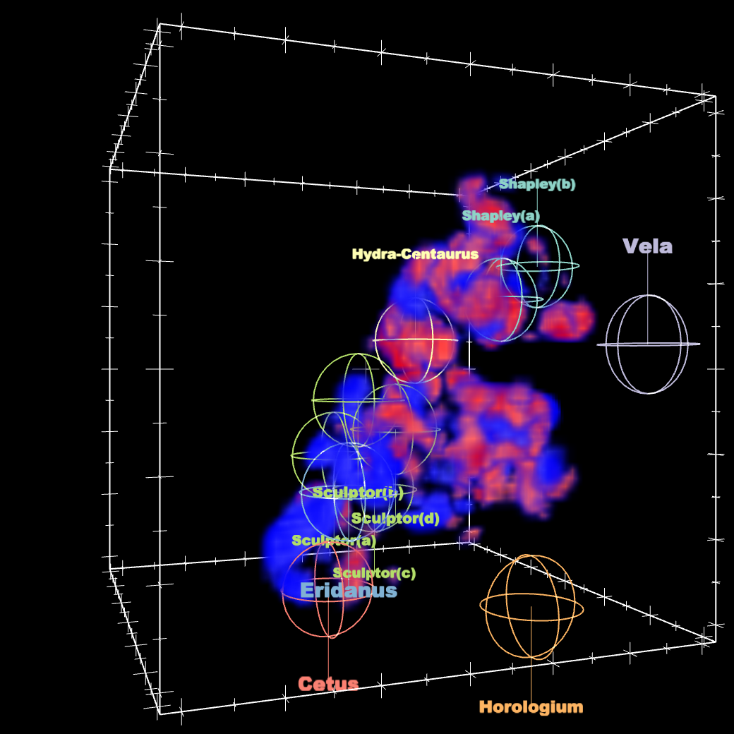
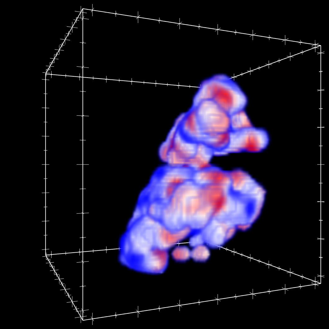
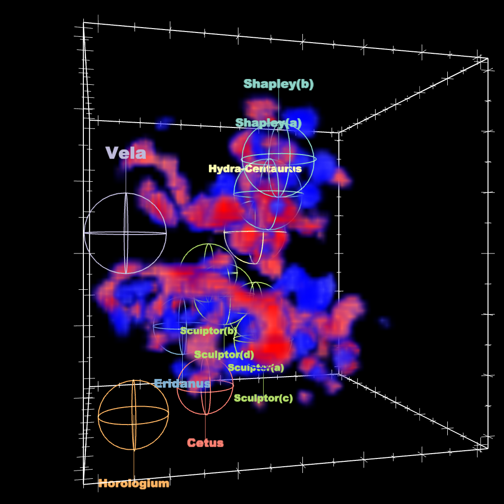 Above: Same as Figure 11, except that we only show gridpoints with extremely positive or negative values of the logarithmic distance ratio. We also label several features of large scale structure. Note the large number of red gridpoints in the direction of structures such as the Shapley and Vela superclusters, and the large number of blue gridpoints in the direction of the Cetus Supercluster. This suggests that there is a "bulk flow" in this volume, which will be explored in future papers (Scrimgeour et al., submitted; Magoulas et al., in prep.).
The full 3D version of this plot can be downloaded here. Adobe Reader version 8.0 or higher enables interactive 3D views of the plot, allowing rotation and zoom. To toggle
the visibilty of individual superclusters in the interactive figure, open the Model Tree, expand the
root model, and select the required supercluster name.
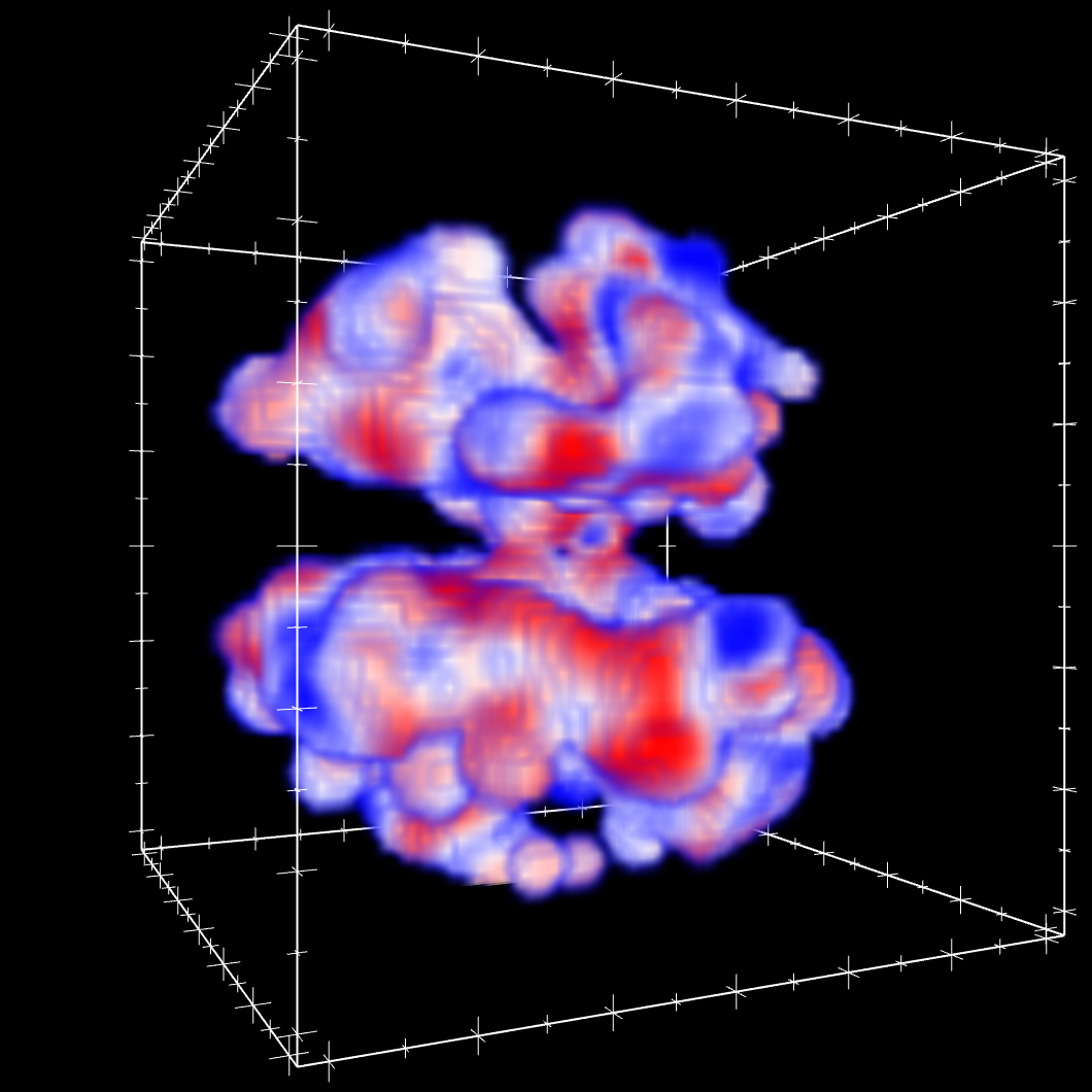
Above: Same as Figure 11, except that we only show gridpoints with extremely positive or negative values of the logarithmic distance ratio. We also label several features of large scale structure. Note the large number of red gridpoints in the direction of structures such as the Shapley and Vela superclusters, and the large number of blue gridpoints in the direction of the Cetus Supercluster. This suggests that there is a "bulk flow" in this volume, which will be explored in future papers (Scrimgeour et al., submitted; Magoulas et al., in prep.).
The full 3D version of this plot can be downloaded here. Adobe Reader version 8.0 or higher enables interactive 3D views of the plot, allowing rotation and zoom. To toggle
the visibilty of individual superclusters in the interactive figure, open the Model Tree, expand the
root model, and select the required supercluster name.
Chris Springob, christopher.springob@icrar.org, Sun, 21 Sep 2014